When you have r=g=b (e.g. (153,153,153)) you will have a colour between black and white, i.e. a shade of grey.
In this part we will study monochrome graphs [because it is easier to understand what happens].
I will only give you single functions. Write it as red component and set green and blue to copy the red one.
First example, a funny fractal-like picture:
If you do (x*y)/255, You will have a kind of diagonal spread, black in the top left corner and brighter in the bottom right one.
But because
modulo 256 is used when it gets too big, you do not see anymore this spread but
some other stange structure. Try it with x*y.
Try then to put multiply it by some constant, like three (x*y*3) or
bigger ones (15,31,...). You will remark that when you are quite near from a
power of two, the picture seems regular but is actually quite chaotic.
Second example, some circles to go on...
If you write x^2+y^2,
you will get the square of the distance from the top left corner, which will
quickly overcome 255. You will see some other (quite unexpected) circles appear.
These other circles are not actually "real", but are caused by the
fact that the program does not calculate all possible places but only the one
that correspond to whole values of x and y (I.e. it does for instance calculate
the pixels (37;0) and (38;0) but nothing between, like (37.5;0).)
Replace now x by
(128-x) and y by (128-y): (128-x)^2+(128-y)^2. You may wonder why I asked
you to do that, since there is no visible change. Actually the only
"real" circle is now at the center and the other are "fake".
If you divide by something, for example 4:((128-x)^2+(128-y)^2)/4, you
will see what I mean. You can see some circles that seem to appear over the
"real" ones. These are the "fakes" that seemed so
"real" before...
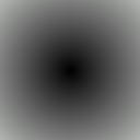
Calculate now the
square root of the previous expression: sqrt((128-x)^2+(128-y)^2)
Now the circles are gone and the colour of pixel is the distance to the center
(Thanks to Pythagore ;-)
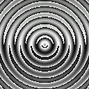
Let's have some
fun with the trig functions. Keep the functions you had before, but put a sine
on it: sin(sqrt((128-x)^2+(128-y)^2)). You should see ugly black and
white rings. This is because the sine function varies between -1 and 1, and -1
is turned into 255 by the modulo.
So try now to multiply it by 127 and add 128 (the [-1;1] range changes now to
[1;255]). Now you can at last see the circles. But how tight they are, they
cause a headache, don't they?
But it is possible to make the gap quite wider, dividing the contents of the
sine function by a constant. Try the following:
sin(sqrt((128-x)^2+(128-y)^2)/5)*127+128. (Now the distance to the center
varies slower than before and the rings are therefore more spaced.
To have some fun,
try now adding y to the whole function (replacing 128):
sin(sqrt((128-x)^2+(128-y)^2)/5)*127+y.
This is like if the whole rings had been a little bent, and overcoming 255 (or
getting under zero) in some places.
Third example, looking in the water.
We'll start with almost the same function than before, the rings, but a lot tighter:
sin(sqrt((128-x)^2+(128-y)^2)*2)*127+128
Save this somewhere (e.g. create a new project) and try the following before we go on:
sin(x/5)*sin(y/5)*127+128
Once you have seen it, let's go back to the previous one, adding
sin(x/5)*sin(y/5)*5 to the contents of the sine:
sin(sqrt((128-x)^2+(128-y)^2)*2+sin(x/5)*sin(y/5)*5)*127+128
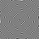
You can now have fun changing some constants. E.g. change the *2 (right after the square root) by *3 and change sin(x/5)*sin(y/5) by sin(x/5)*sin(y/6)..
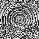
Last example, some abstract art.
Let's go back to our concentric rings:
cos(sqrt((x-128)^2+(y-128)^2)/5)*127+128
Replace +128 by +x+y. You will see the effect you already know.
Now add some
little waves:
(cos(sqrt((x-128)^2+(y-128)^2)/5)+sin(x/5)*sin(y/5))*127+x+y
This makes some funny effect
Multiplying these little waves by (y-100)/100 breaks the symetry and makes the picture more interesting:
(cos(sqrt((x-128)^2+(y-128)^2)/5)+sin(x/5)*sin(y/5)*(y-100)/100)*127+x+y
2.1: Four operators
2.2:
Trigonometric functions
2.3: Min, Max, Modulo, Abs and Neg
2.4: Other functions
3.1: Monochrome
Graphs
3.2: Implicit functions
3.3: Playing with hyperbolic tangents